How we fit a live, audio-driven video diffusion model into 320 ms per chunk on one H100
By Faris Rahman, Machine Learning Engineer
At Ojin we serve conversational video avatars in real time. Our Human Presence model listens to a stream of speech audio and generates video of a person saying it, live. It is an autoregressive video diffusion transformer. Each request produces a chunk of 8 frames, which is 320 ms of video at 25 fps. To stay real time, every chunk has to be denoised, decoded, upscaled and sent in under 320 ms, on one GPU, for the whole conversation.
In October 2026 the model ran on B200s. We wanted it on H100s, which cost less and are easier to get, but on one H100 it was over the 320 ms budget. Over about four weeks we worked through hundreds of ideas on Modal, first on an RTX PRO 6000 and then on a single H100. The model now runs at roughly 270 ms per chunk on one H100, and in November we moved production to H100.
We have Modal to thank for the pace of that work. All of those experiments ran on GPUs that Modal provided on demand, first the RTX PRO 6000 and then the H100. We never had to own or operate the hardware, so the four weeks went into the ideas themselves.
Modal also runs the model in production, on H100s. Each live conversation uses one GPU for the whole conversation. Modal's autoscaling starts containers as conversations come in and removes them when they end. Each container starts from a GPU memory snapshot of a fully warmed process and is ready in seconds. That makes a model this sensitive to warmup and memory practical to serve live and to scale. We are grateful for the partnership.
These are 30 of the optimizations in our serving stack, with what each one does, why it helps and what it bought us.
Some context
The model. Each chunk passes through five stages:
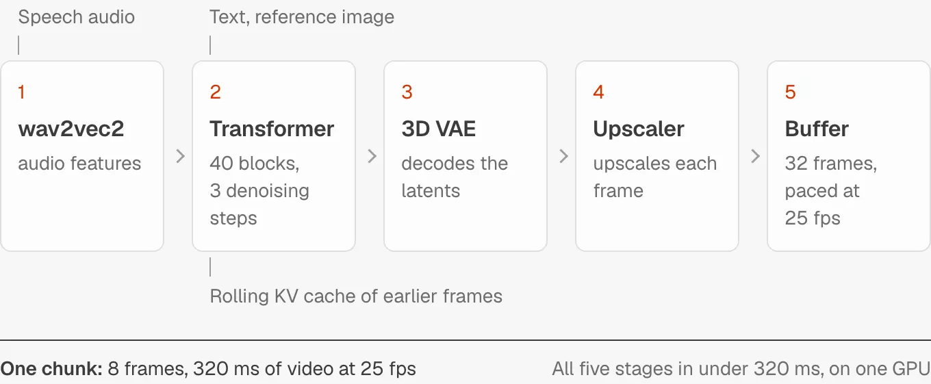
Conditioning comes from text and reference-image cross-attention and from wav2vec2 audio features fed into audio cross-attention. Self-attention reads a rolling KV cache of earlier frames, so the key window is 4 to 7 times longer than the query. The cache advances through a 4-phase cycle, and some phases read longer windows than others.
Each container restores from a Modal GPU memory snapshot of a fully warmed process, with weights loaded, kernels compiled and CUDA graphs captured.
Why bit-exact changes matter. The model is autoregressive: every chunk conditions on the frames before it. Change the last bit of one activation and, a few seconds later, the video differs everywhere. Wherever we could, we built optimizations that leave the output bits unchanged, so that speed and quality could be judged separately.
Part 1: Scheduling and overlap
1. Start the next chunk's first denoising step early
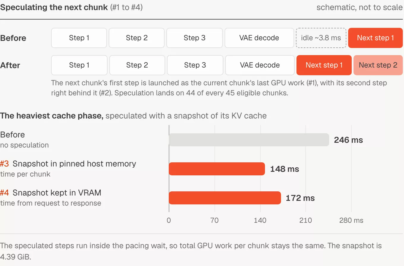
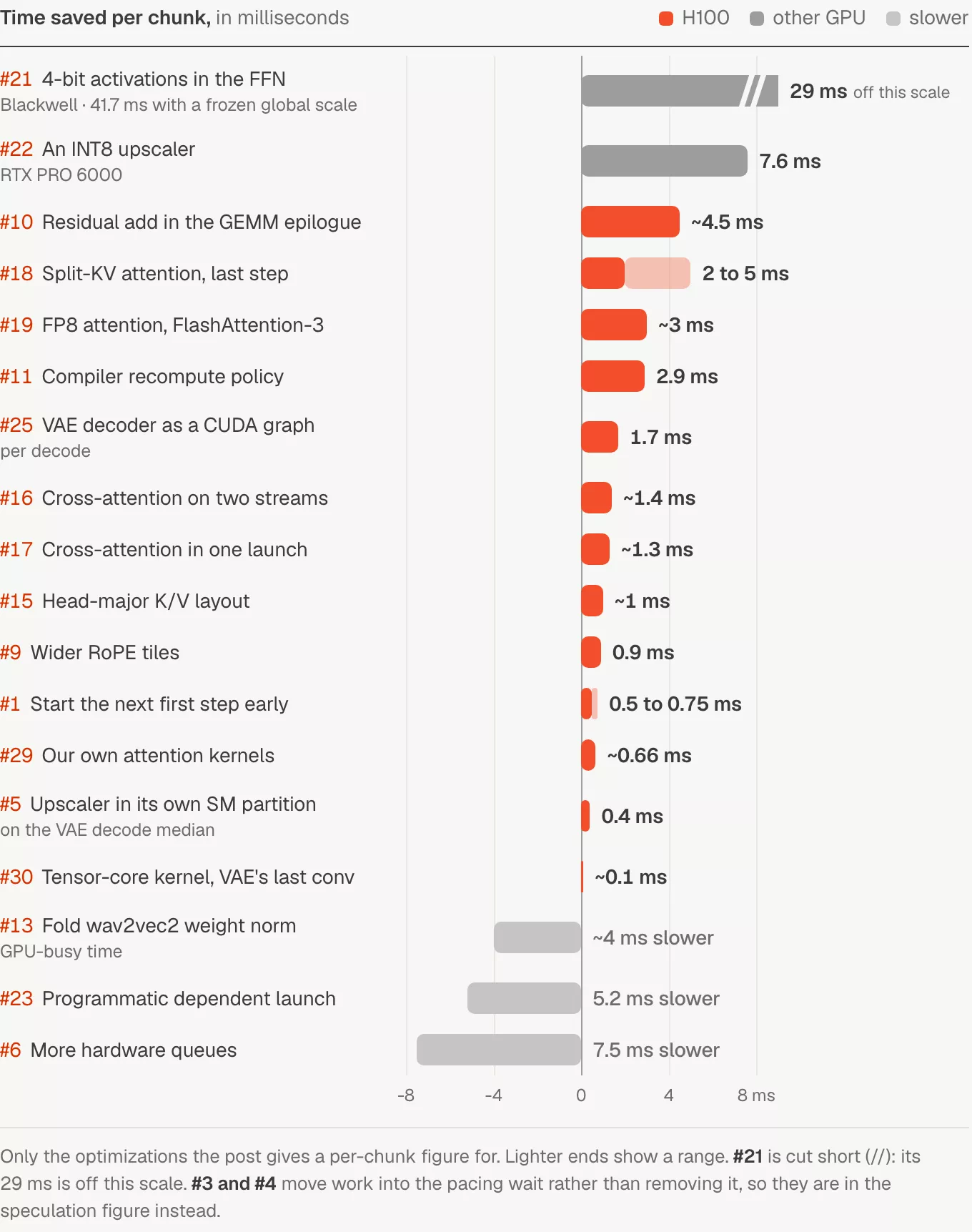
We prepare the next chunk's first step during the VAE decode and launch it as the current chunk's last GPU work. The next chunk's first step gets a 2.35 ms head start, and each chunk takes 0.5 to 0.75 ms less.
2. Speculate two denoising steps instead of one
On the H100 we extended #1 and queue the next chunk's second step right behind its first. In our traces the next chunk's second step starts about 11 ms earlier.
3. Speculate the heaviest cache phase, staged through pinned host memory
Result. Time per chunk fell from 246 ms to 148 ms. The snapshot copy shares PCIe with frame delivery.
What we did. One cache phase compacts the KV cache in place, so a wrong guess cannot be thrown away. The first step's cache slots do not change between two consecutive uses of that phase, so we copy them (4.39 GiB) to pinned host memory before speculating, and restore them on a miss.
Why it helps. The GPU no longer idles before the heaviest phase, and the snapshot costs no VRAM.
4. The same speculation, with the snapshot kept in VRAM
Result. Time from request to response fell from 246 ms to 172 ms, with a 4.39 GiB snapshot in VRAM. The speculated steps run inside the pacing wait, so total GPU work per chunk stays the same.
What we did. We keep the snapshot in GPU memory, which makes it a 3 ms copy inside HBM. It is released on the session's cold chunks, where memory is tightest.
Why it helps. It avoids PCIe traffic on the hot path entirely, so the snapshot never competes with the frames' device-to-host copies.
5. Fence the upscaler into its own SM partition with CUDA green contexts
We confine the upscaler to a 24-SM green context, created with cuGreenCtxStreamCreate and a stream priority. The VAE decode median went from 40.37 ms to 39.97 ms, and the output is bit-identical.
6. More hardware queues: CUDA_DEVICE_MAX_CONNECTIONS=32
By default CUDA maps streams onto 8 hardware work queues, and we raised the limit to 32. In our runs the chunk measured 7.5 ms slower, and GPU-busy time rose from 291 to 296 ms.
7. Fill the attention kernel's last wave with the next GEMM
We split the attention into a body and the tail rows, and the output projection's quantization and GEMM run on a side stream in the SMs the tail leaves free. It made no measurable change in our runs.
Part 2: Kernels
8. Contiguous loads in the RoPE kernels
Result. Each RoPE op is 12 to 23 % faster in isolation; the largest went from 100 to 87 µs. The q/k write went from 62 to 53 µs and the fused norm-plus-RoPE from 64 to 56 µs.
What we did. Our rotary-embedding kernels used to read interleaved (even, odd) pairs with two stride-2 loads and two stride-2 stores. They now load one contiguous tile per head group and split the pairs in registers with tl.reshape, tl.split and tl.join in Triton. The output is bit-identical.
9. Wider RoPE tiles
We process 8 heads per register tile with 8 warps, instead of one head at a time with 2 warps. It saved 0.9 ms per chunk in our kernel benchmark and is bit-exact.
10. Fold the residual add into the GEMM epilogue
Result. About 4.5 ms per chunk in our kernel benchmarks: 8.6, 9.4 and 19.4 µs less per call on the three projections. 191.9 to 183.3 µs for the attention output projection, 192.1 to 182.7 µs for the cross-attention output and 458.6 to 439.2 µs for the FFN down-projection.
What we did. Each transformer block computes x = x + gate * proj(y) three times. We wrote a Triton FP8 GEMM that is bit-exact against the vendor kernel and puts the residual add in its epilogue. It handles the channel-major bf16 residual stream and the bf16 gate that production uses.
Why it helps. It saves a full read and write of the residual stream per projection.
11. Tune the compiler's recompute policy (realize_reads_threshold)
Result. The transformer takes 2.9 ms less per chunk in the pipeline. The transformer's block tail got 5.5 % faster in our benchmark.
What we did. Inductor's realize_reads_threshold decides when a value read by several consumers is stored once and when it is recomputed in each consumer. We lowered it to 2 for the transformer's compiled graphs only, so the residual stream is stored at each block boundary.
12. A channels-last wav2vec2 feature extractor
We switched the convolutional feature extractor to channels-last. It runs in 213 µs instead of 256 µs per call, compiled in isolation, and the output is bit-identical.
13. Fold wav2vec2's weight normalization once, at load time
wav2vec2's positional convolution uses weight normalization, so we fold its effective weight once at load. One kernel of about 0.9 ms per chunk in our profile leaves the audio path, but in our runs GPU-busy time still rose about 4 ms, because the folded convolution took a slower path.
14. Channels-last convolutions in the VAE decoder
The VAE decoder's 3D convolutions run in channels-last layout. Each convolution is 16 % faster in isolation, and the output is bit-exact.
15. A head-major K/V layout for attention
K and V are stored head-major (HND) instead of sequence-major. The gain is 5 to 13 µs per attention call, about 1 ms per chunk, and the output is bit-exact.
Part 3: Attention and cross-attention
16. Run text and image cross-attention on two streams
We fork the text and image cross-attentions in each block onto two streams inside the captured step graph and join them afterwards. In our benchmark that took a block-step from 114.0 to 102.1 µs, about 1.4 ms per chunk, and it is bit-exact.
17. Batch text and image cross-attention into one launch
Both cross-attentions run as one launch with a batch of 2. A block-step went from 114.3 to 103.1 µs, about 1.3 ms per chunk, in our benchmark, bit-exact.
18. Split-KV attention for the final denoising step
Result. 2 to 5 ms less per chunk.
What we did. The final step's self-attention reads up to 13,440 keys. We split the keys into three ranges inside one attention call and merge the results with a log-sum-exp kernel.
Why it helps. Long key windows get more parallelism: 1683 to 1512 µs at 13,440 keys, with outputs within 61 to 62 dB of the original.
19. FP8 attention with FlashAttention-3 on H100
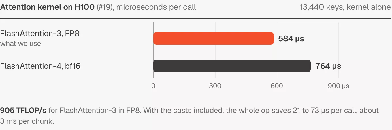
Result. On the kernel alone at 13,440 keys, FlashAttention-3 in FP8 takes 584 µs (905 TFLOP/s), against 764 µs for FlashAttention-4 in bf16. With the casts included the whole op saves 21 to 73 µs per call, about 3 ms per chunk. FP8 copies of K and V need 5.5 to 10 GB of VRAM for every layer (3.99 GB for 29 layer-steps).
What we did. FlashAttention-3 has an FP8 forward pass on Hopper, and it installs cleanly from the PyTorch CUDA 13 index. K and V are written to FP8 once, when they enter the cache.
20. SageAttention2 (INT8 QK, FP8 PV) on H100
We ran SageAttention2's Hopper kernels, which quantize Q and K to INT8 and P and V to FP8, with fp32 accumulation. In our runs, with every kernel on the right stream, it was slower, at 1394 µs against 745 µs for FlashAttention-4.
20b. A note on timing third-party kernels
When we first benchmarked SageAttention2 under CUDA graphs, its launches on the legacy default stream were not captured, which made the timing look better than it was. Time third-party kernels eagerly with CUDA events, and check that a graph replay really recomputes.
Part 4: Precision
21. 4-bit activations in the FFN on Blackwell (NVFP4, W4A4)
Result. 29 ms less per chunk, and 41.7 ms with the frozen global scale. SyncNet lip-sync confidence comes out about 0.17 lower, so check lip sync on your own data.
What we did. On the RTX PRO 6000 (Blackwell), vLLM's NVFP4 GEMM lowers with CUDA 13. We run the FFN with 4-bit activations. The activation global scale is calibrated once and frozen, which makes the quantization token-independent. With a dynamic per-call scale, a moving person would shift the block-scale grid for the static background tokens and make the background flicker.
Why it helps. The FFN up-projection went from 387 to 210 µs and the down-projection from 442 to 215 µs.
22. An INT8 upscaler
Result. 7.6 ms less per chunk on the RTX PRO 6000, with slightly lower image-quality scores on the mouth region.
What we did. The upscaler is a small all-convolutional network with 64-channel 3×3 convolutions. We built an explicit INT8 TensorRT engine with cross-layer equalization, keeping the first conv and the last four in FP16.
Why it helps. On the RTX PRO 6000 it is 32 % faster per frame, at 45.8 dB against FP16.
Part 5: Compiler, graphs and memory
23. Programmatic dependent launch (TORCHINDUCTOR_ENABLE_PDL=1)
We enabled programmatic dependent launch in Inductor. In our runs the chunk measured 5.2 ms slower, and turning it on re-autotuned 179 kernels.
24. Skip TorchDynamo's guard checks on the VAE decode
The VAE decode runs with the same input signature on every steady chunk, so we skip its guard evaluation. The result was below run-to-run noise (about ±2 ms) in our runs.
25. Capture the VAE decoder as a CUDA graph
Result. 1.7 ms per decode in our benchmark, bit-exact. The graph needs 2.5 to 3.5 GiB more persistent memory.
What we did. The VAE decode replays as one manually captured CUDA graph. The graph's private memory pool takes over the eager workspace that the restore-time allocator reserve used to hold, so the reserve shrank from 16 to 12 GB.
Why it helps. It removes per-kernel host dispatch.
26. Reuse dead buffers
Result. About 2.5 GB of VRAM back, at no cost in speed or bits.
What we did. Some per-layer cache buffers are allocated for every layer but are never read during one denoising step: about 2.5 GB in all. We reclaim them.
Part 6: Tuning against vendor kernels
27. Our own FP8 GEMM in Triton on H100
We wrote a Triton TMA FP8 GEMM with row-scaled A, per-tensor-scaled B and the bias in the epilogue, and swept block sizes, warps and stages. In our runs cuBLAS stayed faster at every shape, for example 76 µs against 95 µs for the output projection.
28. FlashAttention-4 tiles tuned for our shapes
We swept query tiles from 64 to 192 and key tiles from 64 to 256 at the windows the model actually reads. A 128 × 192 tile was the fastest at 13,440 keys, 0.7 % faster at 744.0 against 749.5 µs.
29. Our own attention kernels in Triton
A single Triton kernel computes image and text cross-attention together. It takes 67.4 µs against 73.2 µs per call, about 0.66 ms per chunk.
30. A tensor-core kernel for the VAE's last convolution
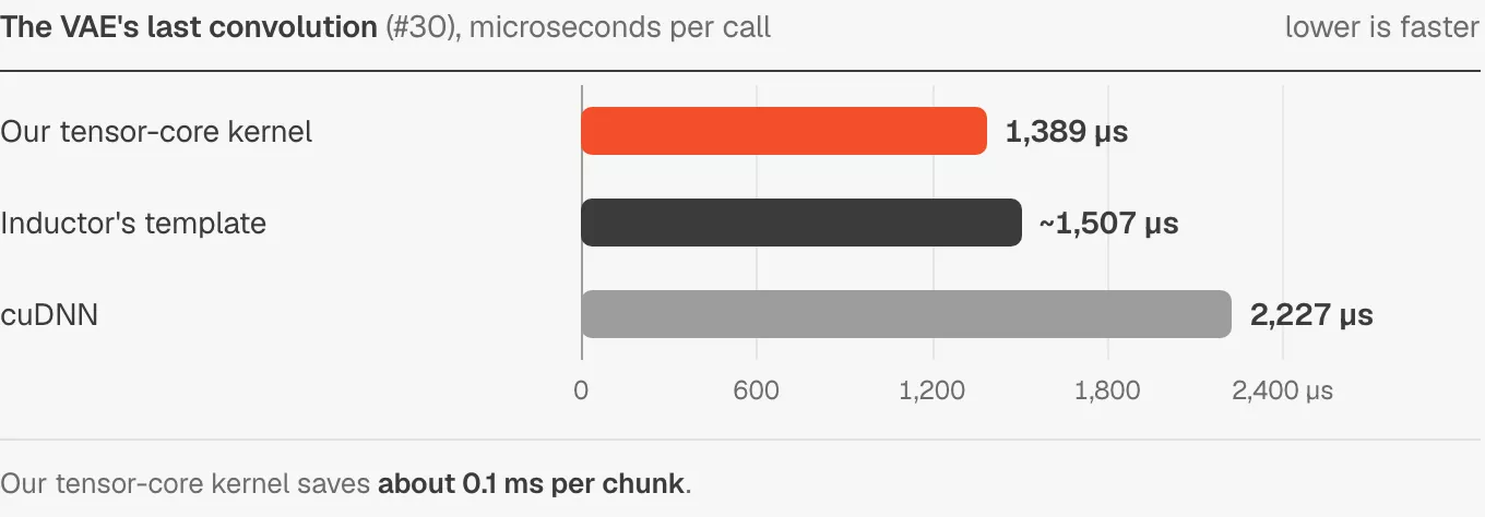
The VAE's final convolution maps 96 channels to 3 (RGB), and we pad the output to 16 channels so that tensor cores can do the work. It takes 1389 µs against about 1507 µs for Inductor's template and 2227 µs for cuDNN, about 0.1 ms per chunk.
What these have in common
At a power cap, removing work beats hiding it. Both GPUs ran at their power limit. The biggest gains came from fewer FLOPs, fewer bytes and lower precision, not only from overlap.
Benchmark inside the real graph. L2 state, SM sharing with other streams and stream semantics under graph capture all change a kernel's behaviour. We measured every change inside the full pipeline.
Bit-exactness belongs to the compiled graph. Changes that touch the compiled graph's structure can change fusion and autotuning decisions. Keeping changes inside opaque custom ops, or outside the graph, kept the output bits stable.
Memory is a budget. CUDA graphs, FP8 copies and snapshots all cost VRAM. The tightest moment is the warmup's autotuning, not serving.
Watch lip sync when you lower precision. For a talking-head model the mouth is where precision shows first, so we checked it on every precision change.
Summary
Running on Modal
All of this runs on Modal. It gave us the GPUs we needed, when we needed them, so our four weeks went into trying ideas and not into setting up hardware. We could test an idea on one kind of GPU, then move to another, without buying or managing either.
Modal also keeps the model running for the people who use it today. Every live conversation needs its own GPU, so the number we need changes all the time. When more conversations start, Modal adds capacity, and when they end, it takes it away again.
A model like ours takes a while to get ready before it can answer. Modal saves it in its ready state, so each new machine starts in seconds. That let us keep our attention on the model itself.